Maze Contest: A Quick Analysis
Time for a tournament arc!
Apr 10, 2021
One of my CS classes this semester runs a semester-long contest to see who can write the fastest concurrent maze solver. Submitted programs are tested on a battery of 7 mazes that may or may not be solvable and a public scoreboard is updated quasi-daily with each competitor’s runtime performance on all the mazes as well as their rank and score. With such a treasure trove of data before my eyes, I could not resist and set out to run some analysis on it.
Parsing and Cleaning the Data
As it is, the scoreboard is simply an HTML table on a web server which needed to be parsed. The good news is that this part of the project was already done. I had been working on a separate project before this to visualize the data from our contest and had been regularly parsing and saving snapshots of the scoreboard with a Cloudflare Worker for a few weeks already, so getting the data was a simple matter of downloading the latest snapshot my worker had saved. However, my worker stores the scoreboard snapshots as serialized JSON objects which are not too convenient for running statistics on. I ended up writing a small Python script to transform all the data into a CSV, ending up with the following table:
| # | name | rank | maze1 | maze2 | maze3 | maze4 | maze5 | maze6 | maze7 | score |
|---|---|---|---|---|---|---|---|---|---|---|
| 1 | * | 1 | 1.100 | 0.108 | 1.468 | 2.469 | 0.330 | 0.380 | 1.159 | 139 |
| 2 | * | 2 | 0.987 | 0.210 | 1.600 | 2.431 | 0.288 | 0.339 | 1.057 | 152 |
| 3 | * | 3 | 3.742 | 0.098 | 10.209 | 6.144 | 0.375 | 1.697 | 5.770 | 168 |
| 4 | * | 4 | 2.202 | 0.268 | 2.587 | 5.421 | 0.363 | 0.494 | 1.859 | 176 |
| 5 | * | 5 | 3.785 | 0.096 | 10.326 | 6.110 | 0.374 | 1.685 | 5.912 | 202 |
| 6 | * | 6 | 3.761 | 0.097 | 10.242 | 6.120 | 0.380 | 1.682 | 5.981 | 210 |
| … | … | … | … | … | … | … | … | … | … | … |
At this point, the data still needed to be cleaned. Not all programs on the scoreboard ran correctly for all mazes, so these entries needed to be filtered out. Since these failing entries also caused the columns end up with non-numerical data, each maze column and the score column also had to be be converted to numerical data.
# Read and filter data
data <- read.csv("./out.csv") %>%
  na_if('err') %>%
  na_if('bad') %>%
  na_if('ovr') %>%
  na_if('FAILED') %>%
  drop_na()

for (i in 1:7) {
  maze <- sprintf('maze%d', i)
  data[[maze]] <- as.numeric(as.character(data[[maze]]))
}
data$score <- as.numeric(as.character(data$score))
Filtering the data brought the number of entries from 155 down to 132 points. Now that we had some pretty clean data, it was time to dive into some statistics!
Maze Runtime Statistics
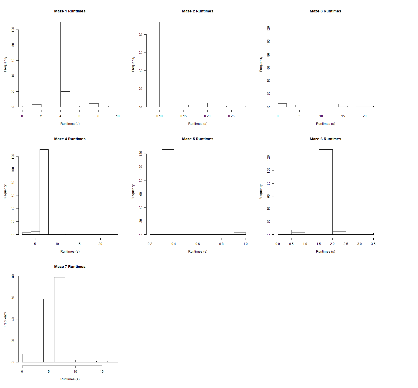
Exploratory data analysis was first performed on the data. This consisted of graphing a histogram and generating some statistics for the runtimes of all 7 mazes.

| Maze # | Mean (s) | SD (s) |
|---|---|---|
| 1 | 3.857 | 0.757 |
| 2 | 0.105 | 0.0234 |
| 3 | 10.262 | 1.860 |
| 4 | 6.367 | 1.623 |
| 5 | 0.385 | 0.037 |
| 6 | 1.697 | 0.291 |
| 7 | 5.947 | 1.147 |
In general, it seems that mazes with greater average runtimes displayed greater standard deviations. This is probably because mazes with greater runtimes are likely larger, unsolvable mazes. This means more variability in how programs may proceed with searching the maze over time and thus more variability in the amount of time a program would take to solve the maze or determine that it is unsolvable.
Despite this, the histograms and standard deviations seem to show that, overall, there is not too much spread in the runtimes for each maze amongst competitors. This seems to indicate that most programs are performing quite similarly to each other on all of the mazes.
While these histograms give a good initial look at the runtimes, it also divorces each program from its performance on all 7 mazes as a whole. To see how each competitor’s program was related to one another, we need to cluster the data.
Clustering the Competition
To make the clusters, each competitor’s maze runtimes was treated as a 7D vector with the runtime for each maze occupying a dimension. The vectors were fed into K-means with 3 centroids which gave the following:
runtime_data <- data %>% select(starts_with('maze'))

# Kmeans
kmeans_res <- kmeans(runtime_data, centers=3)
kmeans_res$centers
Cluster centers:
| # | maze1 | maze2 | maze3 | maze4 | maze5 | maze6 | maze7 |
|---|---|---|---|---|---|---|---|
| 1 | 1.453400 | 0.1904000 | 1.96160 | 3.55420 | 0.3530000 | 0.472400 | 1.377400 |
| 2 | 3.909024 | 0.1013333 | 10.59048 | 6.35104 | 0.3845714 | 1.745048 | 6.128159 |
| 3 | 9.255000 | 0.1880000 | 10.32500 | 22.46000 | 0.6390000 | 1.706000 | 6.007000 |
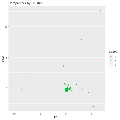
Each data point was also transformed into 2D space for visualization by applying PCA and graphing the first two principal components of each transformed point.
# PCA
pca <- prcomp(runtime_data, center=TRUE, scale.=TRUE)
summary(pca)
Importance of components:
| metric | PC1 | PC2 | PC3 | PC4 | PC5 | PC6 | PC7 |
|---|---|---|---|---|---|---|---|
| Standard deviation | 1.9748 | 1.4750 | 0.65062 | 0.47248 | 0.43497 | 0.24521 | 0.17016 |
| Proportion of Variance | 0.5571 | 0.3108 | 0.06047 | 0.03189 | 0.02703 | 0.00859 | 0.00414 |
| Cumulative Proportion | 0.5571 | 0.8679 | 0.92835 | 0.96025 | 0.98727 | 0.99586 | 1.00000 |

The PCA summary shows that the first two PCs capture about 87% of the variance so the transformation still retains most of the information from when the points were in 7D.
From here, we can begin to characterize our 3 clusters:
Cluster 1: Gotta Go Fast
Cluster 1 consists of 5 points that are spread decently far apart. The cluster’s center shows faster runtimes compared to all other centers on each maze except maze 2.
Overall, this group seems to be comprised of the fastest programs. Due to their spread, the creators of these programs probably took different approaches from each other to design but ultimately still managed to create programs that were able to out-perform most of the other solvers on most of the mazes.
Cluster 2: Most of Us+
Cluster 2 is the largest cluster at 126 data points and also the most densely clustered with only 6 points deviating significantly from the main blob. Compared to the cluster 1 center, cluster 2’s center displays about 2-5x slower runtimes with the greatest difference being in the maze 3 performance (1.96s vs 10.59s).
Almost all of the submitted programs fall in cluster 2 and nearly all of those fall within the main blob. This seems to support the earlier observation from the histograms that most programs in the contest perform very similarly. While the performances of most programs are similar, it is difficult to say whether this similarity in performance is because of similar implementation or because most of us were hitting the same barriers to improvement despite having different methodologies.
Cluster 3: Pluto
The final cluster consists of a single data point, so nothing can be said about spread within the cluster. The centroid cluster shows similar maze performance to that of cluster 2 with 2-4x slower runtimes on mazes 1, 2, 4, and 5.
While this point is far from the cluster 2 blob, it is only the tip of the iceberg. There are 23 failing programs that were initially filtered out and not considered in this analysis. If we had included those data points, setting each point’s missing runtimes to an arbitrarily large value, the graph might have instead shown a fan of points stretching out beyond this one.
Closing Remarks
Ultimately, the data analysis yields a very boring conclusion: most everyone is about the same. While we do have a few outliers, they do not amount to many; over 70% of the class is contained within a single, dense blob.
I also haven’t mentioned how programs are ranked. While you would think it’s based on fastest average time across all mazes, it’s actually based on smallest cumulative rank across all mazes. A competitor’s rank for each maze is summed with smallest summed value corresponding to highest ranker. This means that even if your program significantly out-performs everyone else’s on a large maze, if it is not optimized for a small maze and runs 0.1 seconds slower than everyone else’s, you are ranked last for that maze and drop rank significantly. Ultimately, this means that while our clustering says something about the performance of the programs, it does not say much about their ranking in the contest. While many members of cluster 1 are also high rankers, being in cluster 1 does not guarantee high rank.
Of additional note is that this analysis is only based on a snapshot of the scoreboard at around the time of writing. The contest runs until the end of the semester, and we are free to improve our programs however we like. It is very possible for the clusters and rankings to change as competitors find smarter and leaner ways to solve mazes. Perhaps the everyone blob will scatter; perhaps we will all end up in cluster 1. Only time will tell, but until then, let the maze solver tournament arc continue!
UPDATE 08/19/21: Convert HTML tables and code output to Markdown tables.